Black Scholes Merton Model, Binomial Tree Distribution, Put-Call Parity…….., you must have read or heard about them while exploring the derivatives market. For an trader trying to develop the logical framework of the futures and options, one needs to understand them. But, how did we develop the intuition and the knowledge to express these dynamic movements in mathematical terms. Let us look at a branch of mathematics, an extremely powerful tool, Stochastic Calculus
What is Stochastic Calculus?
Stochastic Calculus is a branch that specifically operates on stochastic processes. So why do we need it? Why can’t we deal the problem with the normal mathematics? To answer this let’s first understand what are stochastic processes.
In all of mathematics, we deal with functions and variables and perform various operations on them. In classical mathematics, we deal with functions with are continuous or you might say follow a well defined trajectory. But what if a variable doesn’t obey a fixed rule? Like in the case of bacterial population growth, or movements in a gaseous molecule? Such processes are called stochastic processes. Therefore, stochastic processes/random process can be defined as family of random variables in a probability space, where index of the family is a function of time.
How did the Stochastic process come to use in financial markets?
The price movement of an asset does not follow a uniform trajectory. In early 1900’s Louis Bachelier presented his thesis on option pricing. In the thesis Bachelier proposed that the stock prices follow a random walk(drawing parallels to Brownian motion). The thesis laid the foundation of what would become stochastic process. Then Norbert Wiener in 1920s and Kiyoshi Ito in 1940s provided rigourous mathematical framework for random walks. Fischer Black and Myron Scholes utilised the framework laid by Wiener and Ito to develop an model of option pricing for European style options in 1973. This gave financial professionals a tool to consistently derive a “fair” price of options, which lead to the prominent rise of quantitative finance.
We’ve journeyed through the intriguing origins of stochastic process and looking at it’s pivotal role in financial markets. While it may have laid the groundwork, it merely scratches the surface of the power and elegance these tools possess. In the blogs that follow, we will dissect critical components, providing clear insights into theorems like Ito’s Lemma, stochastic differential equations and much more.
Option pricing may be considered a multivariate function with the stock price, time to expiration , volatility, strike price and interest rates as the variables then. The Black Scholes Model was introduced in 1973. Developed by Fischer Black, Myron Scholes, and Robert Merton, the model was first published in Black and Scholes’s paper, “The Pricing of Options and Corporate Liabilities,” in the Journal of Political Economy. The formula for prices of European calls and puts on non dividend paying stocks are:
Theoretical Price for call options = PN(d1) –Ke-rTN(d2)
Theoretical Price for Put options =Ke-rTN(-d2) – PN(-d1)
where:
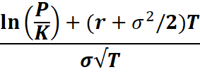
d1=
d2 = d1 – σ√T
where P is the stock price, K is the strike price, r is the risk free rate, N(x) is the normal distribution function
**The model is only applicable to European Style options. Numerical methods like binomial and trinomial distributions are used for pricing of American style options.
Let’s analyse each term in the expression and try to find out what it denotes:
PN(d1): This term represents the expected benefit from owning the stock, weighted by the probability that the stock price will be above the strike price at expiration.
Ke-rt N(d2): This term represents the present value of the cost of exercising the option, weighted by the probability of stock price being higher than the strike price.
Assumptions in Black Scholes Merton Model:
The model assumes the market volatility to be constant throughout.
Buying or selling the options does not incur any transaction costs, commission, or fees.
The stock does not pay dividends during options lifetime.
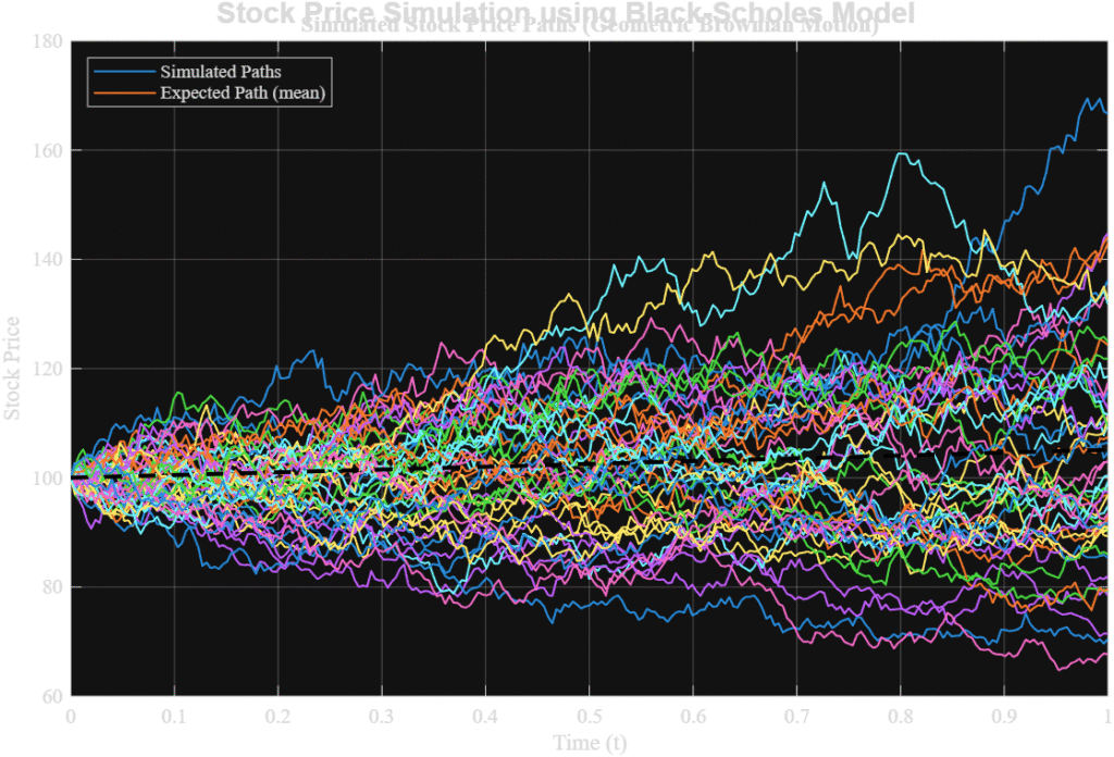
Log-Normal Distribution of Stock Prices: The underlying asset’s price follows a geometric Brownian motion, meaning its continuously compounded returns are normally distributed (and prices are log-normally distributed). This implies continuous price movements with no “jumps.”
The differential equation for the pricing of the model is given as:
dPt = μPtdt + σPtdWt
where Pt is the stock price at time t, μ is the expected return(annualised), σ is the volatility of the stocks return
What should traders take care of?
While the model uses ‘volatility’ as an input, traders cannot predict the future volatility of an asset and hence use implied volatility(IV).
Implied volatility is the market’s expectation of future volatility. It’s derived by taking the actual market price of an option and “backing out” the volatility that the model would have needed to produce that price, given all the other known inputs (stock price, strike, time to expiration, risk-free rate).
Why is this model important?
Well to answer the biggest question, why do we need it.
The answer to it is that the Black Scholes Merton model provides a foundation of the ‘Greeks’ which are crucial in understanding the option pricing and risks associated with the assets.
Applications:
Warrants and Convertible Securities: Companies use the model to value warrants (rights to buy stock at a certain price) and convertible bonds/preferred stock (which can be converted into common stock).
Employee Stock Options (ESOs): The BSM model is widely used in corporate finance to value ESOs for accounting purposes and to design compensation packages.
Risk Management: The model helps financial institutions assess and hedge their risk exposure to various financial instruments by calculating “the Greeks” (delta, gamma, theta, vega, rho), which measure an option’s sensitivity to changes in its input parameters.
Mergers and Acquisitions (M&A): The model helps in valuing complex financial structures often involved in M&A deals.
Real Options Analysis: This is a significant application where the principles of financial options are applied to strategic investment decisions in real assets (e.g., the option to expand, defer, or abandon a project). It provides a more flexible valuation framework than traditional Net Present Value (NPV) analysis by accounting for managerial flexibility.
Understanding what Merton Said?
The Black Scholes model assumed that the stock is non dividend paying. Merton, not long after, presented his model where took into account that the stock pays dividend. But that turned out to be a drawback as it assumed continous dividend pays for the same amount which made it unrealistic. The model follows the same PDE as the above model, except that the amount of continous dividend is added in the equation. Further publications, like Hull and White(1987), Musiela and Rutkowski(1997) and Bos and Vandermark(2002) developed the Black Scholes Model.
Conclusion:
To sum up, the Black-Scholes-Merton model, despite its theoretical assumptions, provides an invaluable framework for anyone engaging with options. Its brilliance lies in democratizing option valuation and, crucially, in giving rise to “the Greeks” – essential tools for understanding risk. For investors, the takeaway isn’t just about plugging numbers into a formula; it’s about appreciating that while BSM gives us a theoretical price, the implied volatility derived from market prices is often the most critical factor. By understanding both the model’s logic and the market’s dynamic interpretation of volatility through IV, investors can approach options trading with greater insight and a more informed strategy.